The Mean-Variance Efficient-Portfolio Frontier
- A mean-variance efficient portfolio \(\w^{\text{mv}}(\bar\mu)\) is the portfolio that shows minimum-variance
for given target return \(\bar\mu\). It solves the problem
\(\begin{eqnarray*} \frac{1}{2}\var(\w) &\to& \min_w\\[1em] \text{s.t.}\quad \w'\eins &=& 1,\\[0.2em] \w'\bmu &=& \bar\mu. \end{eqnarray*} \)
- Since the variance of any portfolio \(\w\) can be decomposed into
\( \var(\w) = \var(\w^{\text{gmv}}) + \var(\w-\w^{\text{gmv}}), \)
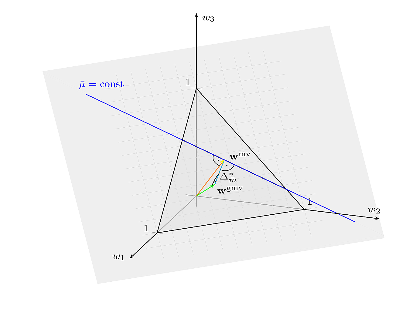
searching for the mean-variance efficient portfolio among all portfolios with a given return \(\bar{\mu}\) is equivalent to searching for the minimum-variance portfolio transaction \(\Delta_{\w} = \w-\w^{\text{gmv}}\) among all transactions with a given expectation \(\bar m = \bar\mu-\bar\mu(\w^{\text{gmv}})\)\(\begin{eqnarray*} \frac{1}{2}\var(\Delta_{\w}) &=& {\Delta}'_{\w}\Sigma\Delta_{\w} \,\to\, \min_w\\[1em] \text{s.t.}\quad {\Delta}'_{\w}\eins &=& 0,\\[0.2em] {\Delta}'_{\w}\bmu &=& \bar m. \end{eqnarray*} \)
- We are looking for a portfolio transaction that bridges the return difference \(\bar m\) and has minimum-variance, i.e., which is orthogonal (in the covariance sense) to all transactions among portfolios with equal return expectation.
Min-Var Transaction
We denote \({\Delta}^*_{\bar m}\) the solution of the above optimization problem. Then, the mean-variance efficient portfolio \(\w^{\text{mv}}(\bar\mu)\) corresponding to the target return expectation \(\bar\mu = \bar\mu(\w^{\text{gmv}})+\bar m\) is given by\( \w^{\text{mv}}(\bar\mu) = \w^{\text{gmv}} + {\Delta}^*_{\bar m}. \)
Min-var efficient portfolio \(\w^{\text{mv}}\) and the min-var efficient transaction \({\Delta}^*_{\bar m}\).
Mean-Variance Efficient Frontier
The mean-variance efficient frontier is the location of mean-variance efficient portfolios \(\w^{\text{mv}}(\bar\mu)\) for all possible target returns \(\bar\mu\).The mean-variance efficient frontier is a straight line. It is true that
\(\begin{eqnarray*} {\Delta}^*_{k\bar m} &=& k {\Delta}^*_{\bar m},\\ {\Delta}^*_{\bar m_1 + \bar m_2} &=& {\Delta}^*_{\bar m_1} + {\Delta}^*_{\bar m_2} \end{eqnarray*}\)
Since it is a straight line, the entire frontier is spanned by any pair of two mean-variance efficient portfolios. In particular, if we know the global minimum-variance portfolio and another mean-variance efficient portfolio which corresponds to the return expectation \(\bar\mu_1=\bar\mu(\w^{\text{gmv}})+\bar m_1\) the entire frontier is defined by\( \w^{\text{mv}}(\bar\mu) = \w^{\text{gmv}} + \frac{m}{m_1}{\Delta}^*_{\bar m_1},\quad m = \bar\mu-\bar\mu(\w^{\text{gmv}}) \)