Returns
- Consider a universe of \(n\) securities with prices \(x_{0,i}\), that are observable at the beginning of the investment period, at \(t=0\).
Prices at the end of the period, at \(t=1\), are \(x_{1,i}\). These prices are not observable before \(t=1\). - Paying \(x_{0,i}\) at \(t=0\) brings ownership of one unit of security \(i\). Over the investment period, this investment translates
into a holding that is worth \(x_{1,i}\). Ownership, however, entitles the investor to receive dividends or coupons or any other
cash flow that the security provides over the investment horizon.
Let us denote the cash flow per unit of investment \(d_i\). - Investing an amount of EUR \(K\) in security \(i\) translates into a value of \(K (1+r_i)\) at the end of the holding period.
- At the point where the investment decision is made (\(t=0\)), the returns \(r_i\) are not known and, thus, random numbers.
- Let us write the holding-period returns \(r_i\), \(i\in\{1,\dots,n\}\), of the securities under consideration into one joint vector
\(\r\) defined as
\( \r = \left(\begin{array}{c} r_1\\ r_2\\ \vdots\\ r_n \end{array}\right) \)
Simple Return
The simple return of security \(i\) over the investment period -- also called holding-period return -- is defined as\( r_i = \Frac{x_{1,i}+d_i-x_{0,i}}{x_{0,i}} =\Frac{x_{1,i}+d_i}{x_{0,i}}-1. \)
Portfolios
- If we have a given amount of money \(K\) at our disposal, we can either invest the whole amount in one of the \(n\) securities, or we can spread the investment over these securities. Then we have to decide which fraction should be invested in each of the individual securities.
- Portfolios are those vectors in the \(n\)-dim weight space that satisfy the equation
\( \w'\eins=1. \)
Such a linear equation defines a hyperplane in \(\R^n\) which is orthogonal (Euclidean right angle) to the vector \(\eins\). - Pure investments of the entire amount \(K\) in only one of the available securities are part of the portfolio plane since they
constitute the basis vectors of the \(\R^n\).
Investing 100% in security \(1\) corresponds to the weight vector \(\p_1\) and investing 100% in security \(i\) corresponds to the vector \(\p_i\), respectively,\( \p_1 = \left(\begin{array}{c} 1\\ 0\\ \vdots\\ 0 \end{array}\right), \quad\quad \p_i = \left(\begin{array}{c} 0\\ 0\\ \vdots\\ 1\\ \vdots\\ 0 \end{array}\right) \left.\begin{array}{c} \\ \\ \phantom{\vdots}\\ \leftarrow\text{position }i\\ \phantom{\vdots}\\ \\ \end{array}\right. \)
Thus, all pure investments are elements of the portfolio plane. - Investing an amount of \(w_i K\) into security \(i\) leads to owning \(\frac{w_i K}{x_{0,i}}\) units of this security.
- So investing a portfolio \(\w\) at time 0 translates into a value of
\( \sum_i\Frac{w_i K}{x_{0,i}}(x_{0,i}+d_i) = K \sum_i w_i(1+r_i) \)
at time 1. - In a general portfolio \(w\) we allow negative weights. A negative weight \(w_i\) means that we short-sell security \(i\),
which generates an inflow of \(w_i K\) at time \(t=0\).
In such case, security \(i\) serves as a financing vehicle. The costs for this financing are uncertain, since at the end of the investment period we have to compensate the buyer of the security with repaying \((1+r_i)w_i K\). - Long-only portfolios lie within the polyhedron spanned by the pure investments.
Portfolio
We call \(\w\), the vector that contains the weights \(w_i\) (= relative portion) invested in the individual securities a portfolio, if the weights sum exactly to 1, i.e.,\( \w = \left(\begin{array}{c} w_1\\ w_2\\ \vdots\\ w_n \end{array}\right),\quad \sum_i w_i= \w'\eins=1, \quad\text{with } \eins = \left(\begin{array}{c} 1\\ 1\\ \vdots\\ 1 \end{array}\right). \)
The Portfolio Plane
Illustration of the portfolio plane in \(\R^3\).
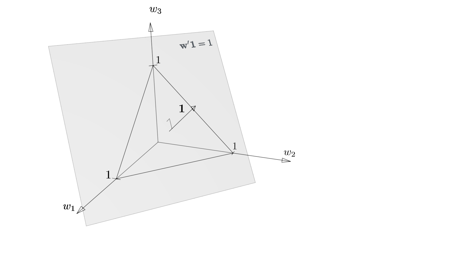
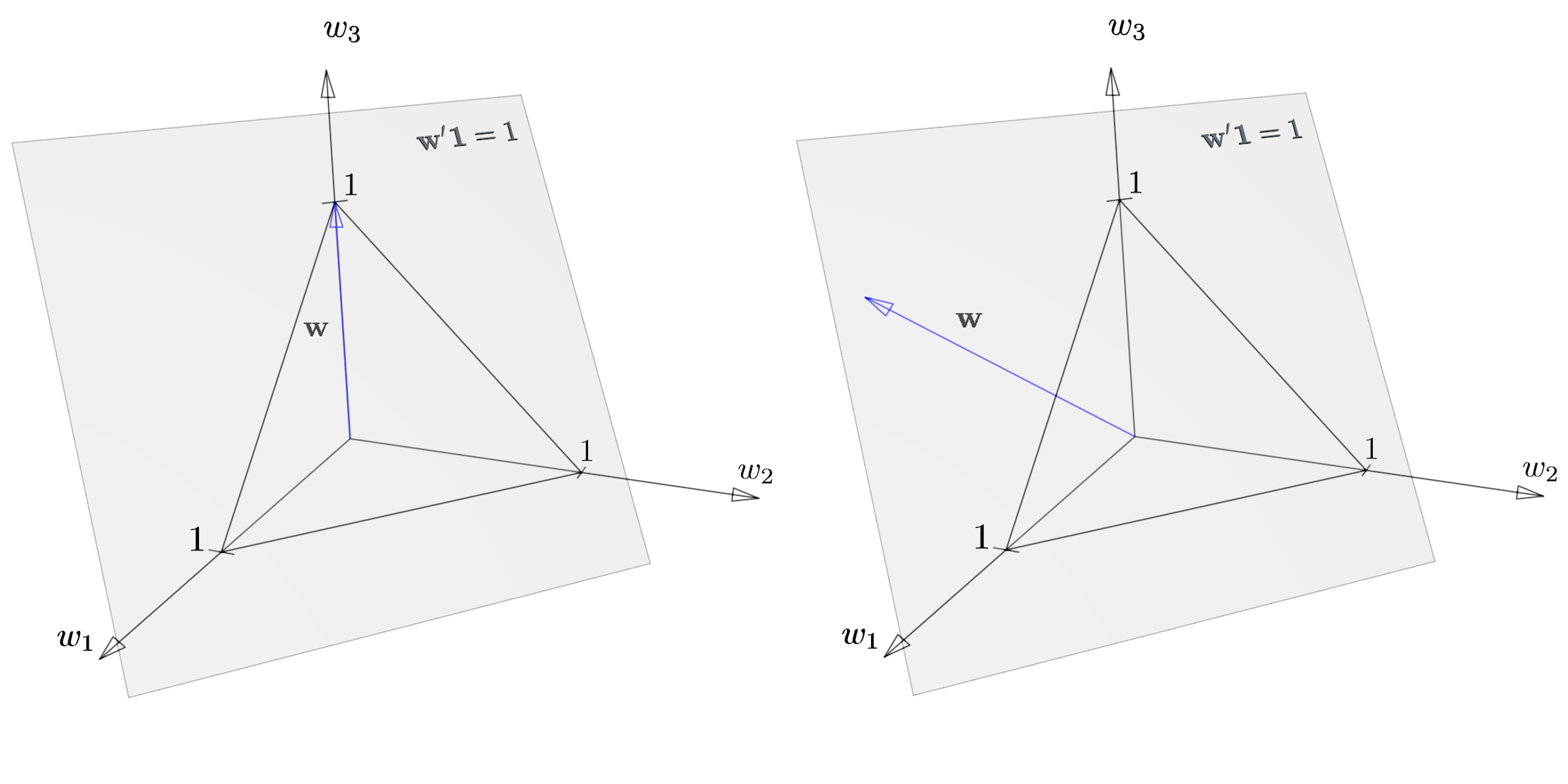
Illustration of the portfolio plane and a weight vector that corresponds to a pure investment in the 3rd security (left figure) and some general portfolio (right panel).
Portfolio Return
The holding-period return of a portfolio \(\w\) is\( r_{\w} = \sum_i w_i r_i = \w'\r \)
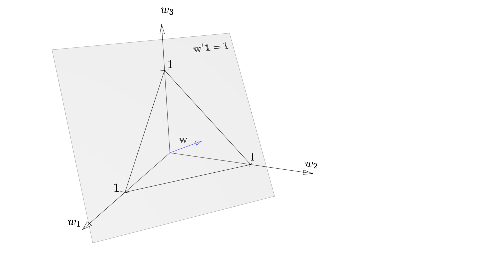
Long-only Portfolio
We call a portfolio \(\w\) a long-only portfolio, if all weights are non-negative\( \w = \left(\begin{array}{c} w_1 \geq 0\\ w_2 \geq 0\\ \vdots\\ w_n \geq 0 \end{array}\right),\quad \sum_i w_i= \w'\eins=1. \)
In \(\R^3\), portfolios inside the triangle spanned by the three pure investments have all weights non-negative, i.e., they are long-only. The illustrated portfolio \(\w\) is one example for a long-only portfolio.
General Return Combinations
- The most general way to talk about investment in such a universe of securities is a linear return combination.
If we relax the constraint that weights must sum to 1, then a return combination is just an arbitrary linear combination of returns.
Thus, any vector \(\w\in \R^n\) can be seen as a return combination, with components \(w_i\) as weights. While portfolios and long-only portfolios constitute only special subsets of the \(\R^n\), return combinations cover the complete \(n\)-dim space. - The interpretation of such return combinations in an economic context, however, is not always straight forward. Since weights do not necessarily sum to 1, it needs to be clarified what the conditions are under which the residual weight (positive or negative) is invested. I.e., in such a case the \(n\)-dim universe of securities is not the entire investment space and there, apparently, exist some investment alternatives or financing opportunities outside this universe which need additional specification.
- Self-financing investments or long-short investments are return combinations that are not part of the portfolio plane but have obvious
interpretation.
These are return combinations with weights summing to zero. In such a combination, the proceeds from short-selling some of the securities
exactly cover the costs for purchasing others.
Since they are self financing, we do not need to make assumptions on investment opportunities outside the \(n\)-dim investment universe, which usually is necessary to interpret general return combinations.
Sometimes, self-financing investments are called long-short portfolios. However, according to our definition of what a portfolio is, self-financing combinations are not portfolios.
Return Combinations
Return combinations are general vectors in the weight space\( \w = \left(\begin{array}{c} w_1\\ w_2\\ \vdots\\ w_n \end{array}\right). \)
The associated linear combinations of returns\( r_{\w} = \sum_i w_i r_i = \w'\r \)
has no straight-forward economic interpretation and needs to be treated with care.Portfolio Transactions
- A portfolio transaction is the joint change in asset weights that is necessary for moving from an initial portfolio to some target portfolio. Portfolio transactions are self financing. I.e., the proceeds from reducing weights of some of the constituents exactly matches the additional investment in other stocks. Transaction costs are not regarded.
- In portfolio optimization, we often argue with hypothetical transactions. If I can show that for a given portfolio there exists no transaction such that the resulting portfolio is more attractive than the given portfolio, this portfolio is a hot candidate for an optimum.
Portfolio Transactions
A portfolio transaction \(\Delta_{p_1,p_2}\) is the return combination which characterizes the changes in portfolio weights necessary to move from the initial portfolio \(p_1\) to portfolio \(p_2\),\( \Delta_{p_1,p_2} = p_2-p_1. \)
Portfolio transactions are self financing, i.e.,\( \Delta_{p_1,p_2}'\eins = p_2'\eins - p_1'\eins = 0 \)